
History and Examples of Numerical Methods
A short history
Numerical methods have a long and varied history, dating back thousands of years to the development of ancient counting systems. However, the modern era of numerical methods began in the 17th century with the development of methods for solving differential equations by Isaac Newton and Joseph Raphson.
During the 18th century, the French mathematician Joseph-Louis Lagrange developed interpolation methods for approximating the values of functions. Later in the 19th century, the German mathematician Carl Friedrich Gauss developed methods for solving systems of linear equations, which are still widely used today.
The 20th century saw significant advances in numerical methods, particularly with the advent of electronic computers. The development of the first electronic computer in the 1940s led to the rapid development of numerical methods for solving a wide variety of problems.
During this time, numerical methods were applied to a wide range of scientific and engineering problems, including the design of airplanes, the simulation of weather patterns, and the analysis of financial data. The development of numerical methods also played a key role in the development of the fields of computational science and scientific computing.
Today, numerical methods continue to play a critical role in scientific research and engineering design. The development of new methods and algorithms, along with advances in computer hardware and software, are driving new advances in a wide range of fields, from climate modeling to drug design.
Examples of Numerical Methods
Analytical methods rely on mathematical equations to obtain exact solutions for problems. They are used for relatively simple problems that can be solved by hand, but their application is limited to problems that have well-defined mathematical formulas.
Numerical methods, on the other hand, use algorithms to obtain approximate solutions for problems. They are used for complex problems that cannot be solved by hand or for which an exact solution is not available. Numerical methods are particularly useful for problems that involve large amounts of data, complex systems, or non-linear behavior.
In simple terms, analytical methods provide exact solutions, but are limited in their application to relatively simple problems, while numerical methods provide approximate solutions for more complex problems.
For Example:
Using Numerical Method
Problem: A ball is thrown from a height of 10 meters with an initial velocity of 20 meters per second at an angle of 30 degrees to the horizontal. Ignoring air resistance, what is the maximum height the ball reaches, and how long does it take to reach the maximum height?
Solution:
To solve this problem, we can use the equations of motion for projectile motion, which can be expressed in terms of the horizontal and vertical components of the velocity and the acceleration due to gravity.
The initial velocity of the ball can be resolved into its horizontal and vertical components as:
vx = v cos(theta) = 20 cos(30) = 17.32 m/s vy = v sin(theta) = 20 sin(30) = 10 m/s
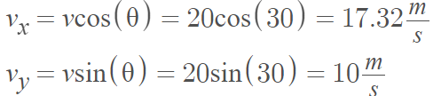
where v is the magnitude of the initial velocity, theta is the angle of the initial velocity.
Using the equation for the vertical displacement of a projectile, we can find the maximum height reached by the ball:
h_max = (vy^2)/(2g) + h0
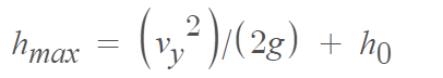
where g is the acceleration due to gravity and h0 is the initial height.
Plugging in the values, we get:
h_max = (10^2)/(2*9.8) + 10 = 15.1 meters

To find the time taken for the ball to reach the maximum height, we can use the equation for the vertical component of velocity:
vy = v0y – gt
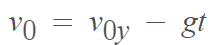
where v0y is the initial vertical velocity and t is the time taken to reach the maximum height.
At the maximum height, the vertical velocity of the ball is zero, so we can solve for t:
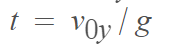
Plugging in the values, we get:
t = 10 / 9.8 = 1.02 seconds
Therefore, the maximum height reached by the ball is 15.1 meters, and it takes 1.02 seconds to reach the maximum height.
Using analytical method
The problem of a ball being thrown from a height of 10 meters with an initial velocity of 20 meters per second at an angle of 30 degrees to the horizontal can also be solved using analytical methods.
We can use the equations of motion for projectile motion, which can be derived using the principles of calculus and physics.
The horizontal and vertical components of the displacement of the ball can be given by:
x = v0 cos(theta) t y = h0 + v0 sin(theta) t – (1/2) g t^2

where v0 is the magnitude of the initial velocity, theta is the angle of the initial velocity, t is the time elapsed, h0 is the initial height, and g is the acceleration due to gravity.
To find the maximum height reached by the ball, we can find the time at which the vertical component of the velocity is zero. This occurs at the maximum height, where the ball starts to fall back down.
The vertical component of the velocity can be given by:
vy = v0 sin(theta) – g t
Setting vy equal to zero and solving for t, we get:
t = v0 sin(theta) / g
Substituting this value of t into the equation for the vertical component of the displacement, we get:
y_max = h0 + (v0 sin(theta))^2 / (2 g)
Plugging in the values, we get:
y_max = 10 + (20 sin(30))^2 / (2 * 9.8) = 15.1 meters
To find the time taken for the ball to reach the maximum height, we can substitute the value of t into the equation for the vertical component of the displacement:
y = h0 + v0 sin(theta) t – (1/2) g t^2
At the maximum height, the displacement of the ball is equal to the maximum height, so we can solve for t:
t = (v0 sin(theta)) / g
Plugging in the values, we get:
t = (20 sin(30)) / 9.8 = 1.02 seconds
Therefore, using analytical methods, we find that the maximum height reached by the ball is 15.1 meters, and it takes 1.02 seconds to reach the maximum height.
A further insight
A simple reminder…
When using numerical methods to solve mathematical problems, it is important to understand that the results obtained will be approximate rather than exact. This is because numerical methods involve using algorithms to obtain an estimate of the solution, rather than solving the problem exactly.
The accuracy of the results obtained using numerical methods depends on several factors, such as the size of the problem, the complexity of the problem, the number of iterations used in the algorithm, and the precision of the computer used for the computation.
In general, as the size and complexity of the problem increase, the accuracy of the results obtained using numerical methods decreases. Therefore, it is important to carefully choose the appropriate numerical method and algorithm for the problem at hand, and to use the appropriate computational resources to obtain the best possible accuracy.
Another important consideration when using numerical methods is the issue of numerical stability. Some numerical methods may be unstable, meaning that small errors in the input data or the algorithm can result in large errors in the output. Therefore, it is important to carefully analyze the stability of the numerical method used and to take steps to ensure that the algorithm is stable.
Overall, when using numerical methods, it is important to carefully consider the accuracy and stability of the results obtained, and to take steps to ensure that the algorithm is appropriate for the problem at hand. With careful consideration and appropriate use, numerical methods can provide powerful tools for solving complex mathematical problems.
CHECKPOINT
- What is the main difference between analytical methods and numerical methods?
a) Analytical methods provide exact solutions, while numerical methods provide approximate solutions
b) Analytical methods use algorithms, while numerical methods rely on mathematical equations
c) Analytical methods are used for complex problems, while numerical methods are used for simple problems
d) Analytical methods are used for problems with well-defined mathematical formulas, while numerical methods are used for problems that cannot be solved analytically - Which of the following is an example of a problem that can be solved using numerical methods? a) Solving a linear equation
b) Finding the derivative of a function
c) Simulating the behavior of a complex system
d) Integrating a function - What is the main advantage of numerical methods over analytical methods?
a) Numerical methods can provide exact solutions
b) Numerical methods are faster than analytical methods
c) Numerical methods can be used to solve more complex problems
d) Numerical methods are more accurate than analytical methods - Which of the following is an example of a numerical method?
a) Differentiation
b) Integration
c) Newton-Raphson method
d) Lagrange interpolation - Which of the following is not a factor that affects the accuracy of numerical methods?
a) Size of the problem
b) Complexity of the problem
c) Number of iterations used in the algorithm
d) Type of analytical method used - Which of the following is an example of an application of Numerical Methods in Engineering?
a) Designing a bridge
b) Writing a computer program
c) Creating a marketing campaign
d) Painting a portrait - Which of the following is an example of an application of numerical methods in finance?
a) Calculating mortgage payments
b) Creating a business model
c) Designing a new investment product
d) Writing a financial report - Which of the following is a limitation of analytical methods?
a) They can only be used for simple problems
b) They are slower than numerical methods
c) They can only provide approximate solutions
d) They cannot be used for problems that cannot be expressed in terms of mathematical formulas - Which of the following is an example of an application of numerical methods in physics?
a) Analyzing historical events
b) Writing a novel
c) Simulating the behavior of a particle accelerator
d) Creating a work of art - Which of the following is a common issue in numerical methods that can affect the accuracy of the results?
a) Numerical stability
b) Analytical complexity
c) Algorithmic instability
d) Mathematical precision
Answers:
- a
- c
- c
- c
- d
- a
- a
- d
- c
- a